Load the libraries and avoid conflicts, and prepare data
# Load libraries used everywherelibrary(tidyverse)library(patchwork)library(mulgar)library(ggdendro)library(fpc)library(tourr)library(colorspace)library(ggbeeswarm)library(ggthemes)library(conflicted)conflicts_prefer(dplyr::filter)conflicts_prefer(dplyr::select)conflicts_prefer(dplyr::slice)
🎯 Objectives
The goal for this week is work on a realistic clustering problem.
🔧 Preparation
Make sure you have all the necessary libraries installed.
Exercises:
Risk taking behavior of tourists in Australia
Most of the time your data will not neatly separate into clusters, but partitioning it into groups of similar observations can still be useful. This is the case for the survey data here, that examines the risk taking behavior of tourists. The risk data was collected in Australia in 2015 and includes six types of risks (recreational, health, career, financial, safety and social) with responses on a scale from 1 (never) to 5 (very often). It isone of the examples in the book “Market Segmentation Analysis: Understanding It, Doing It, and Making It Useful” by Sara Dolnicar, Bettina Grün and Friedrich Leisch. The data can be obtained using the following code:
Using the tour, examine the data, and explain where there are separated clusters, linear or non-linear dependencies.
b. What method is going to partition this data best?
How do you think \(k\)-means would partition this data? What about Wards linkage or single linkage? Why wouldn’t model-based be recommended?
c. Fit the \(k\)-means clustering.
Using \(k=7\) fit the model, and examine the results with a tour.
It’s pretty difficult to see how it has partitioned the data. It has definitely created a cluster of small values but it’s not clear whether the cluster of the larger values are concentrated on different variables.
It still divides the data more messily than anticipated. Cluster 4 though does have small values on all variables, and cluster 5 has moderately small values on all variables. These are the low risk groups. Cluster 7 has high values on most variables, and is a high risk group Cluster 2 seems to have high values on Recreation, and low values on other variables. So it might be considered a cluster of high recreational risk takers. Now your turn to describe the other clusters.
d. Conduct hierarchical clustering.
Use Euclidean distance with Wards linkage to cluster the data and plot the dendrogram. How many clusters are suggested by the dendrogram?
Compute the cluster metrics for the range of cluster numbers between 2 and 7. Which \(k\) would be considered the best, according to within.cluster.ss? Why not be concerned about the other metrics?
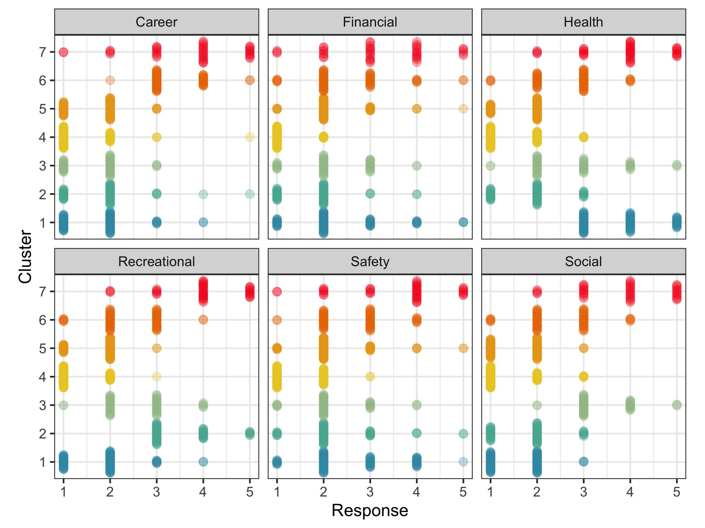
Make a plot of the cluster summary statistics, like slide 11 of week 11 to examine how clustering with different numbers of clusters partitions the data.
d. Conduct \(k\)-means clustering with a range of \(k\).
Fit \(k\) ranging from 2 through 7. Compute the cluster metrics. Which \(k\) would be considered the best, according to within.cluster.ss? Why not be concerned about the other metrics?
Make a plot of the cluster summary statistics, like slide 11 of week 11 to examine how clustering with different numbers of clusters partitions the data.
e. Which is the best result?
Have a conversation with your tutor and class members about which result, or some other might be the best to use for, say, and ensuring that there are enough tourist opportunities for all types of preferences.
👋 Finishing up
Make sure you say thanks and good-bye to your tutor. This is a time to also report what you enjoyed and what you found difficult.